Section 0: Introduction

What follows is a visual guide for anyone curious about the Large Scale Structure of the Cosmos, what we can learn by mapping it, and how we can simulate its formation on a computer.

The Large Scale Structure (LSS) of the universe is a fascinating subject of study for astrophysicists and cosmologists. It refers to the distribution of galaxies and matter on a larger scale than individual galaxies or galaxy groups, with patterns extending up to billions of light years. These structures are formed and shaped by gravity, which pulls galaxies and matter together to create rich and complex patterns, resembling a cosmic web. Studying LSS provides astronomers with important insights into the formation and evolution of the universe as a whole.

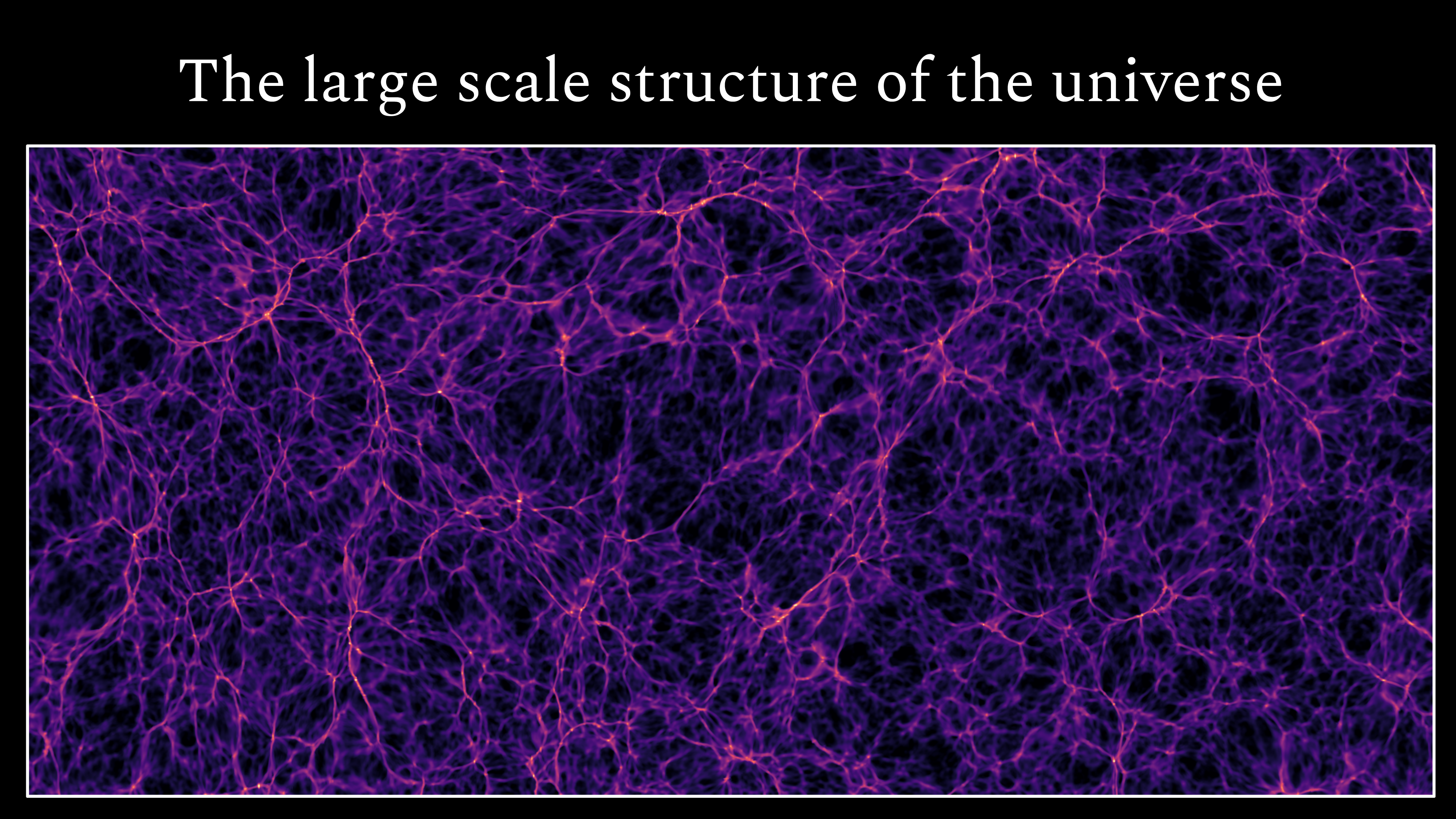Figure 0: Filamentary structures of intergalactic gas spanning tens of Megaparsecs, produced by the Nyx Simulation Suite.

Studying LSS allows cosmologists to measure the strength of gravity in the universe, as they can measure galaxies at different distances and times in the universe’s history, revealing that gravity has been attracting more matter together over time. Furthermore, LSS provides information about dark energy, the mysterious pressure driving the expansion of the universe, which is known to slow down the process of gravity creating large structures. As the universe accelerates in its expansion, matter takes more time to come together due to the increased distance. By studying the growth of LSS over time, astronomers can gain knowledge about how the relative strengths of gravity and dark energy may themselves be changing as the universe evolves.

In this article, we will explore the methods used to map the composition of the nearby universe and the techniques used to simulate the formation of the large scale structure of the cosmos as a whole.

Section 1: Cosmic Cartography

Figure 1: A 3D map of galaxies in the local universe (z<0.15), reconstructed using galaxy spectra by the Sloan Digital Sky Survey.

The simplest way to see this cosmic structure for real is to make a map of the local universe. Figure 1 shows a map of galaxies in the nearby universe up to a distance of about two billion light years away. Each point is a galaxy and the Milky Way (which contains Earth) is at the center. The web-like distribution of galaxies on large scales can be easily seen by eye.

As the universe expands, light traveling through the universe expands as well. As light expands, its wavelength gets longer and consequently looks redder. Galaxies at large redshifts are further away from Earth which means that the light from those galaxies has taken longer to reach our telescopes and thus has spent more time expanding and getting redder. Astronomers have precisely studied the colors of nearby galaxies so they can use this cosmological reddening information to estimate the distance to galaxies based on the color of light they observe.

The variable z is used to quantify this “redshift”, it describes the scalar factor by which the wavelength has expanded by. For example a galaxy at redshift 0.15 is observed at a wavelength 15% longer than when it was emitted.

Nearby galaxy maps like this are extremely useful for understanding the physics of our universe.

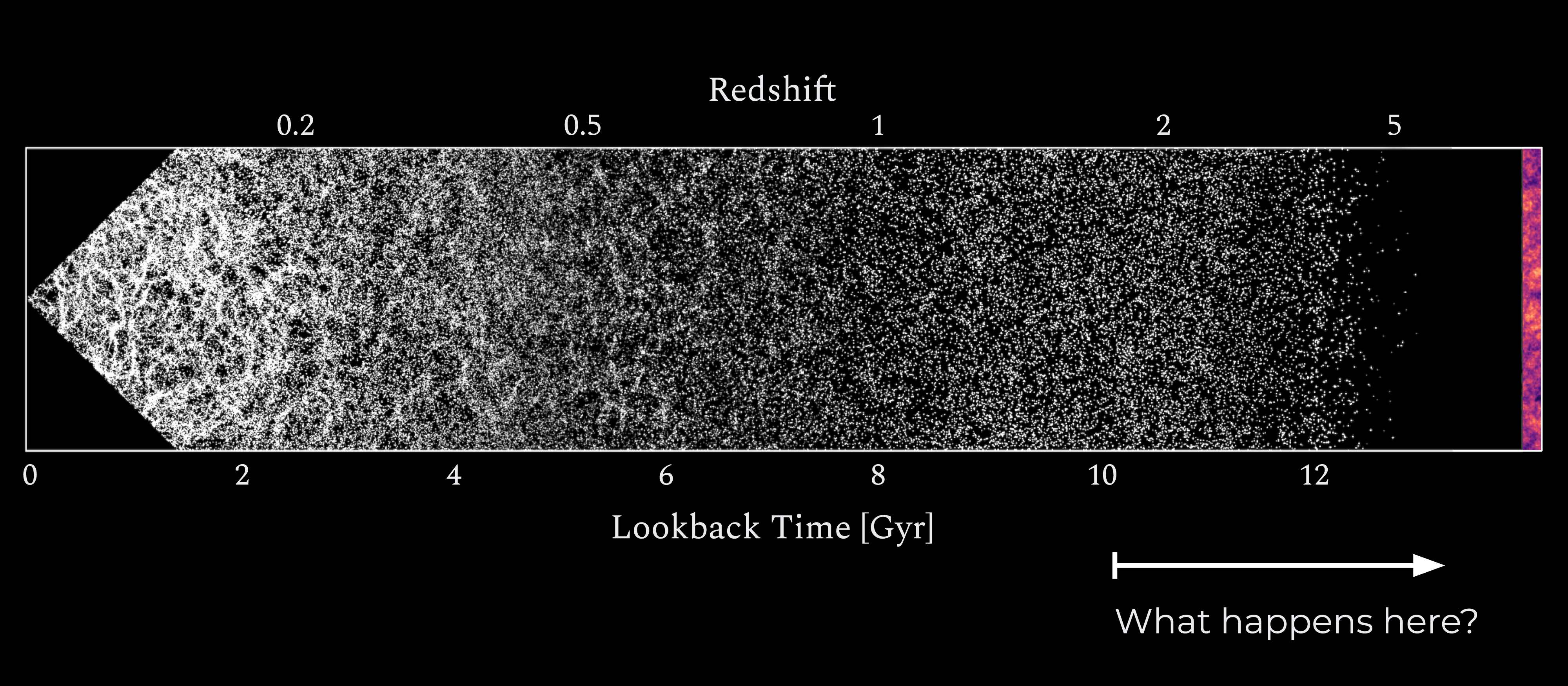Figure 2: A deeper map of galaxies in the more distant universe (z<5), reconstructed using galaxy and quasar spectra by the Sloan Digital Sky Survey, adapted from a figure made by mapoftheuniverse.net showing the cosmic microwave background in the distance.

Two billion lightyears may sound like a lot (and it is!), but the universe is much bigger. As we look further away and further back in time, it becomes more and more difficult to find visible galaxies. As you can see in figure 2, the density of observable galaxies falls off for distances further than z=5 (ie. 500% redder) To map the universe beyond here, astronomers will need to be creative.

It may be hard to see distant galaxies, but a handful of quasars are still visible. Quasars are supermassive black holes at the centers of galaxies. Unlike the dark supermassive black hole in the center of the Milky Way, quasars are some of the brightest objects in the universe. They consume infalling matter so fast that the disk of gas and plasma orbiting around them heats up and glows with the light of a trillion stars. Some of these extreme quasars are so powerful that they can shine 10 or even 100 times brighter than their host galaxies.

Figure 3: Light from a distant quasar is absorbed by intergalactic gas clouds on its way to earth.

Knowing the location of these quasars is interesting, but there are not enough of them to form a complete enough map. Fortunately, the light which reaches us from these distant quasars encodes a lot more information.

As this ancient quasar light travels through the universe, it frequently encounters clouds of intergalactic gas (like that shown in figure 0). As the light enters these gas clouds, certain wavelengths are absorbed and others pass through freely.

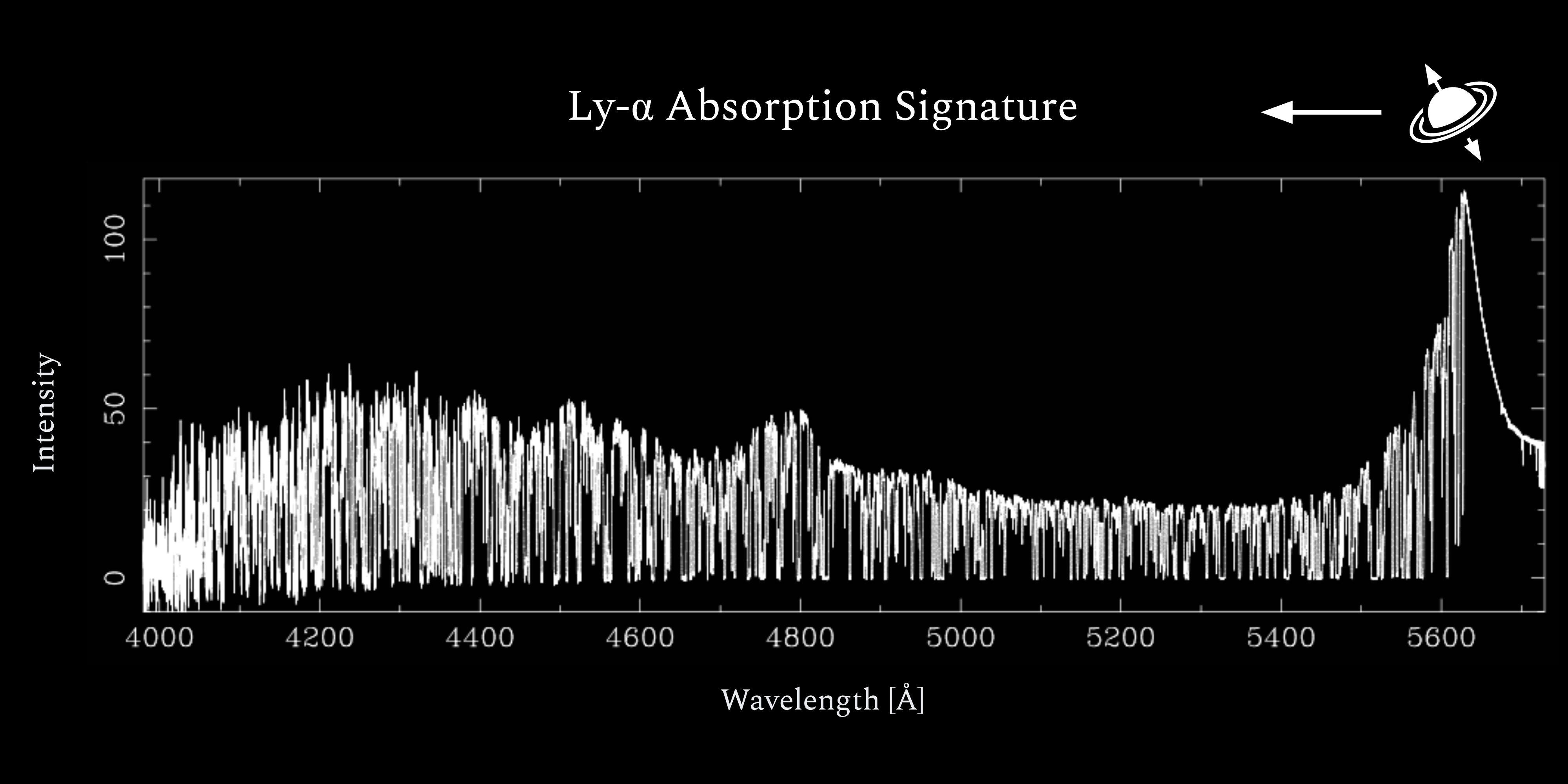Figure 4: High resolution (FWHM ~ 6.6 km/s) spectrum of a quasar at z = 3.62, taken with the Keck High Resolution Echelle Spectrometer (HIRES). Data from Womble et al (1996).

The absorbed wavelengths of light are well known, they are associated with the energy transitions of the element hydrogen, which makes up the majority of these clouds. When the light from a quasar passes through one of these clouds, this wavelength is effectively subtracted from the quasars spectra. You might think of this like a piece of colored glass where if you shine light of all colors (ie. white light) through the glass, orange light might be absorbed but red, yellow, green, blue, purple light pass through the glass freely.

As the remaining light travels through space, the universe continues to expand and stretch the light with it. Every color/wavelength in the quasar’s spectra is stretched individually, so some light which passed through a cloud before may now be absorbed. This is like if the yellow light passes through a first piece of glass but is then stretched out to look orange (i.e. redder than yellow) and is then absorbed by a second piece of glass.

So as the quasar light travels through the universe, the history of all the gas clouds it has encountered along the way is imprinted in the spectra. With nothing in the way, a quasar’s spectra should be relatively smooth, so astronomers can use the sections that appear to be missing to infer the location of the gas clouds it passed through.

Figure 5: Surveying many distant quasars and Lyman-break galaxies allows us to reconstuct an approximate map of the gas ocacity in the distant universe which we can use for statistical analysis.

Modern telescopes can probe the ancient universe with unprecedented precision and depth. Specifically built facilities survey the sky year-round and have mapped millions of these distant quasars and captured their spectra. Using the combination of these spectra, we can construct a map of gas clouds in the distant universe. Figure 5 shows how a set of spectra from distant galaxies and quasars can be used to reconstruct a map of the shadow cast by these web-like gas clouds.

Section 2: Analysis Pipeline

These maps of the cosmos can be used to study the evolution and underlying physics of our universe. The current large-scale structure of the universe is shaped by the parameters of a given cosmological model, as well as initial conditions. By comparing accurate observed galaxy/cluster maps with high-fidelity simulated model universes we can thus constrain the parameters of our cosmological model, for example: the nature of dark matter and dark energy, the history of inflation and reionization in the early universe, and the mass of neutrino particles.

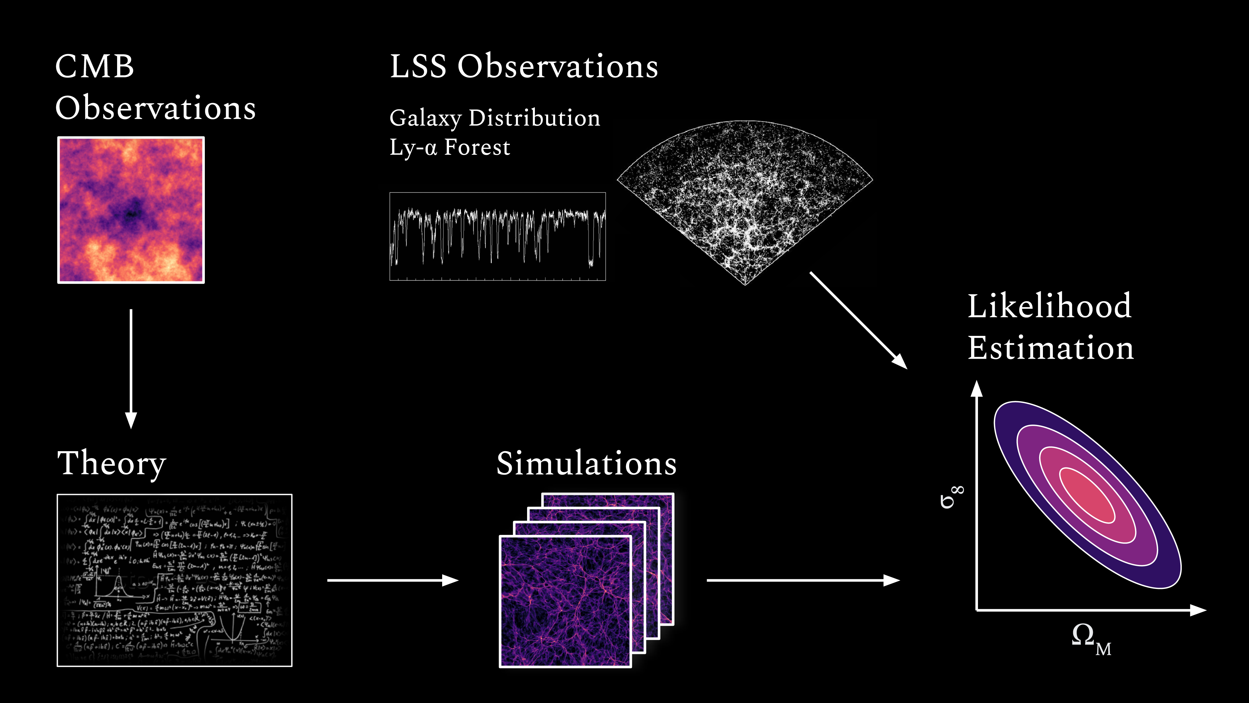Figure 6: Data analysis pipeline for obtaining constraints on cosmological parameters from observations of cosmic structure.

These constraints are found by comparing the statistics of the observed, real universe with a large set of simulated universes. Researchers can change physical properties of the universe when running simulations to see how varying parameters like the density of matter or the strength of dark energy affect the structures that emerge. Finding the parameters of the actual universe then becomes a matter of finding which of these simulated universes is most similar to what researchers observe in reality.

This is not a matter of getting a universe which exactly matches our own, where you could point out some recognisable feature like the Milky Way or Andro (or even yourself). Rather, it is an issue of getting the virtual universe to match the real one statistically. Certain measurable statistical properties of the universe depend on these underlying physical parameters .

In practice, researchers do not need to get these parameters to exactly match the real universe either. With enough sample, simulated universes, researchers can extrapolate the true values based on the correlation between the statistics and the physical parameters. Even so, this analysis will require producing an astronomical number of these simulated universes.

Section 3: Digital Universes

To be able to derive the cosmological constraints discussed above, we need fast and accurate techniques for simulating model universes. Hydrodynamic cosmological simulations are remarkably powerful tools for studying the formation of structure in the universe but require extreme computational resources. Full-physics cosmological simulations are among the most expensive simulations run at supercomputing centers, requiring tens of millions of CPU-hours.

To get an understanding of how these simulations work, we will break down the basic components of the algorithm: gravity and fluid mechanics.

Dark Matter and Gravity Simulation

The overwhelming majority of matter in the universe is what’s called ‘dark matter’. The influence of dark matter has been observed in many different contexts, from the orbital speeds of stars within galaxies to gravitational lensing around galaxy clusters. While Physicists may be unsure what exactly dark matter isAstronomers agree about its presence and influence.

Extensive research has suggested that dark matter is cold and pressureless. Unlike ordinary, visible matter which often collides with itself, dark matter seems to be collision-less. The only influence dark matter has on the universe seems to be via gravity.

Video 1: Simulation of self-gravitating dark matter particles forming structure.

The classic way to model dark matter is using what’s known as an N-Body simulation. This involves some number, N, of particles which can move about a region of space. These particles interact with one another via gravity, attracting towards each other with a force proportional to the inverse square of their distance.

Figure 7: Dark matter structure can be simulated using an N-Body simulation in an expanding spacetime. Many particles gravitationally attract eachother while the frame they inhabit is slowly stretched out.

To model the expansion of the universe, we can include some parameter, a, which defines the scale at a given time. This scale factor increase with time and is used to calculate the effective distance between two points from their comoving (ie. non-expanding) distance. Effectively this means the force of gravity between points gets weaker over time as their effective distance becomes greater.

Appliction 1: Self-gravitating dark matter particles in an expanding spacetime. (You must hold your mouse in the center of the frame for it to animate)

Modeling the universe using this N-Body approach reproduces the web-like filament structures that astronomers have observed.

Visible Matter and Fluid Simulation

There is over five times as much dark matter in the universe as ordinary matter, but (as its name suggests) astronomers have no way to see it. So while dark matter represents the overwhelming majority of the attractive drive behind structure formation, simulations of dark matter alone do not contain all of the information relevant to what can actually be seen.

To simulate the kinds of structure that can be observed by our telescopes, we must also simulate the ordinary (non-dark) matter. Unlike dark matter, ordinary matter is collisional (for instance, you cannot pass your hand through the table). This means that we have to add some new features to our simulation technique to capture the properties of ordinary matter.

The ordinary matter which inhabits the space between galaxies forms a gas. Much like the gasses you’re familiar with here on earth, this intergalactic has some pressure and temperature which affects how it moves. Such a gas will behave like a fluid (note there is a difference between ‘fluid’ and ‘liquid’), it flows much like wind and can even produce turbulence.

Video 2: Evolution of cosmic structure including baryon hydrodynamics. View is 10 Mpc wide, taken from the TNG100 simulation.

As shown in Video 2, this fluid-like behavior of gas produces a much more diverse and interesting structure than the dark matter-only filaments shown in Video 1. You can see the formation of turbulent, spiral clouds which will seed the formation of galaxies and eventually stars. But also between these newborn galaxies are nebulous tendrils of diffuse gas, these are the structures that can be seen with our telescopes.

Simulating this fluid behavior presents a unique challenge, so we will break down the key components of the common methods. In principle it would be possible to use a similar N-body scheme, only modifying the code such that these gas particles could collide and bounce off one another. However to accurately capture the pressure and density of such an N-Body gas, an enormous number of particles would be needed and it would be incredibly inefficient to run on any computer.

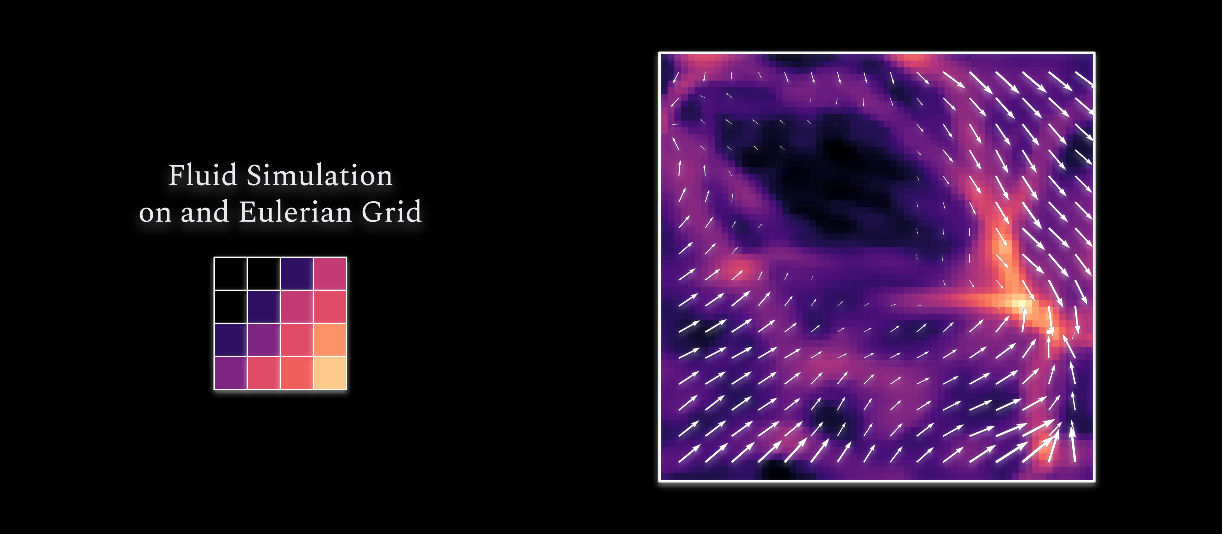Figure 8: The density of intergalactic gas modeled using a grid for the density and velocity fields.

Instead, the gas can be modeled using what’s called a cellular automata. Figure 0 shows a grid of density values where brighter regions are denser. If you are accustomed to thinking of gasses in terms of gas particles, you might think of this density field as encoding the average number of particles per unit volume inside each grid cell.

Each grid cell has some variables associated with it representing the fluid’s average properties within it. For the purposes of these simulations, these properties are the gas density, temperature, and bulk velocity. The grid is updated iteratively to evolve the fluid forward in time. The values in a given grid grid cell at a given time are based on the values of it and its neighbors at the time just before.

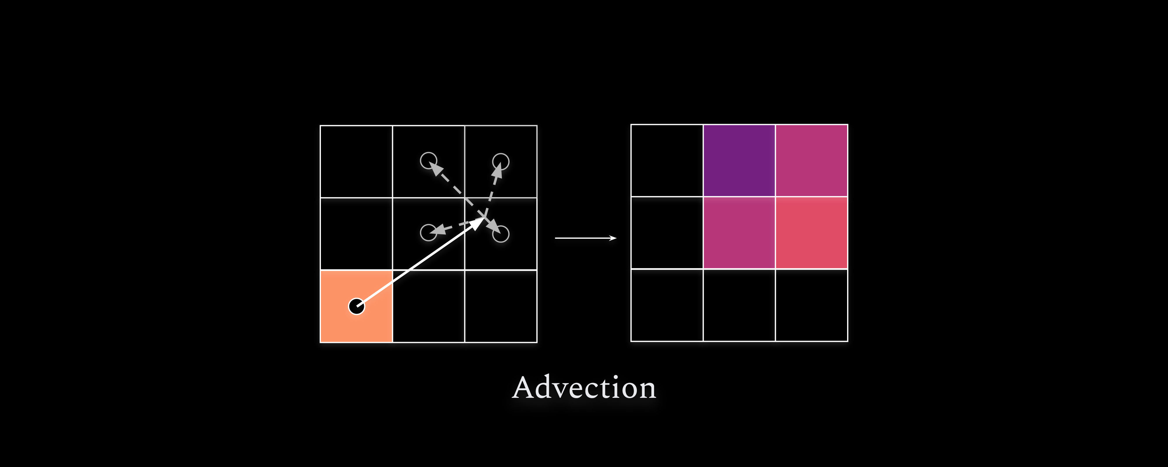Figure 9: Fluid transport (ie. Advection) on an Eulerian Grid is done by distributing the density in given cell to the cells nearest the tip of the velocity vector extending from the start cell.

The velocity of the fluid describes how the fluid should be moving, so the density at a given place ought to be transported according to the velocity there. This is called Advection and in practice it involves updating the density values of the neighboring cells additively based on the direction of flow and density of a given cell, as shown in Figure 9.

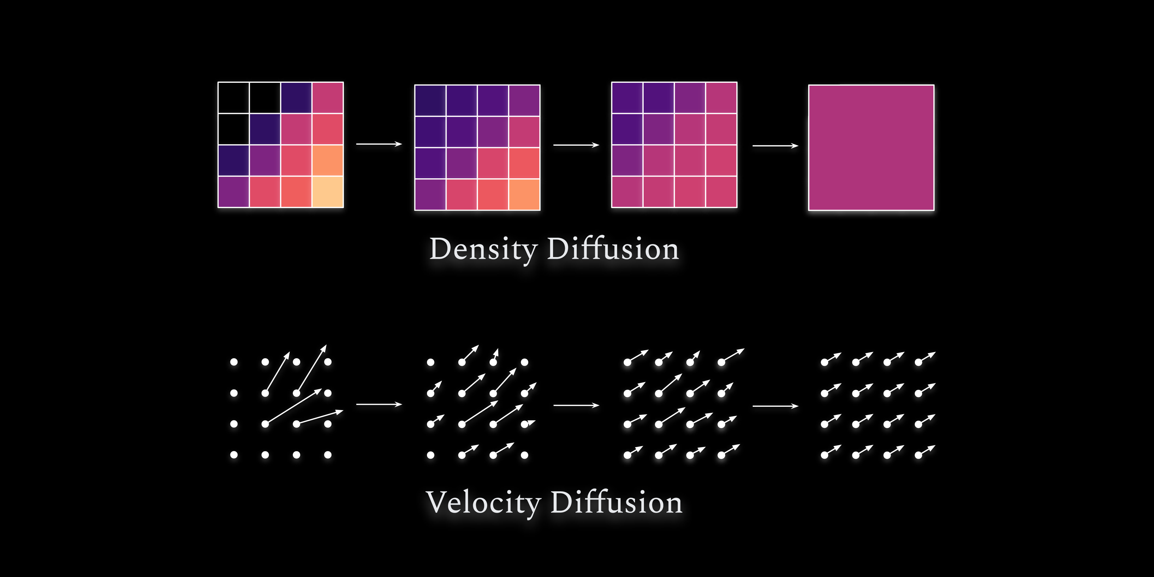Figure 10: Density Diffusion and Fluid Viscosity on an Eulerian Grid are modeled similarly by diffusing a each field slightly each timestep using convolution with some discrete gaussian kernel.

Any good fluid also has some diffusion - if you release gas in one corner of a room, it will eventually make its way to the other side of the room via random motion even without any wind. A good fluid simulation will also include viscosity, the friction that counteracts any shear flow and tends to make the velocity point in the same direction.

These two properties can actually be modeled very similarly. Density diffusion involves updating a local neighborhood of cells each timestep so that they all converge on the average of their neighbors. But viscosity can actually be modeled by doing the exact same process for the velocity vectors so they all align as time goes on. These processes are sketched in Figure 10.

Combining these three processes alone (advection, diffusion, and viscosity) allows us to make a surprisingly realistic fluid model. The interactive application below uses these principles to animate a fluid flow model. You can click and drag with your mouse to make the fluid move.

Appliction 2: Combining the above concepts yields a visually striking fluid model. Click and drag to induce flow.

The fluid model above is a good proof of concept, but it is crude and inaccurate. We can improve the accuracy by just making the grid cells smaller. The cells in the application below are half as wide as in the one above. Since this means we need four times as many cells to fill the same amount of space and therefore four times as much computer memory to store each iteration of the fluid. The speed of the algorithm which advects the fluid depends on the number of cells it has to consider in a non-linear fashion. Having to consider four times as many cells means the computer takes eight times as long to update each frame.

In theory, we could keep shrinking the size of the cells until we had a perfect fluid. But in practice this becomes increasingly expensive, so researchers settle for some small-enough grid with just enough resolution to capture the phenomena they care about.

Appliction 3: Increasing the grid’s cell density improves the fluid’s realism. Click and drag to induce flow.

To accurately simulate the formation of cosmic structure, we can couple these two simulation techniques together. The N-Body dark matter simulation can exert some force on the ordinary matter fluid simulation, pulling the fluid towards the dense clusters.

The fluid models above are really more like water and less like intergalactic gas. A better model of gas would take into account things like density and temperature, whereas the toy models above treat everything as equal. To improve this model we would need to model the thermodynamic properties of the gas and use them to calculate an outward pressure that would come from the hotter cluster (as visible in the video above). But this simple advection-diffusion captures most of the important aspects.

Initial Conditions

The final remaining question is the initial conditions of our simulation. How we initial the density in our model will have as much effect on the resulting structure as the physical parameters we are trying to measure. For instance, if we started with everything perfectly uniform then no structure would form at all. There needs to be some kind of initial randomness to see the growth of structure.

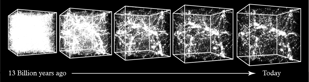Figure 11: Simulation of gravity in an expanding Universe. As time goes on (left to right) the universe itself is expanding so any given box within the universe gets bigger. In reality this effect is much more exaggerated. Adapted from an figure by the National Center for Supercomputer Applications (NCSA).

But not all randomness is created equal. Consider the plot below showing different random fields, you will notice that they vary pretty substantially in smoothness. These are known as gaussian random fields, and each of these them is consistent with the expectations we would have for our initial conditions of our universe. Using different values for this initial smoothness would result in radically different structures down the line. Beginning with a field of entirely uncorrelated noise (like the leftmost field) would lead to entirely lots of very small structures whereas using huge smooth blobs (like the rightmost) would produce massive galaxy clusters with enormous voids in between.

Figure 12: Observations of the CMB provide constraints on the initial conditions of the overdensity fluctuations as modeled by a guassian random field.

Fortunately, these initial conditions are something that astronomers can measure. Modern radio telescopes (both in space and on the ground) have mapped the cosmic microwave background (CMB) in great detail. While it is impossible to know the exact initial conditions that led to the exact structures that astronomers observe, observations of the CMB have measured the smoothness of this primordial noise to a high confidence. Researchers can use these constraints to initialize their simulations to produce the most faithful realizations of the Cosmos.